
4.4 The Phillips curve: The inflation–unemployment dilemma
Can we buy lower unemployment by paying with more inflation?
The Phillips curve: Useful as a thinking tool, dangerous as a fixed menu.
Let’s be honest: if somebody offered a choice between a little inflation and a little unemployment, the argument would be fierce but manageable. Turn a dial, accept the price and you’re done. Unfortunately, the relationship doesn’t stay put. Sometimes you get inflation and unemployment together, with no discount for the bundle.
Today I want to discuss the Phillips curve. It isn’t a regularly published indicator like CPI, or something you can buy. It is a representation of an economic relationship: how labor-market pressure is associated with wage or price changes, depending on the version. It organizes mechanisms and assumptions. It doesn’t promise a policy combination that works forever.
Where it began: British wages and unemployment 📚
In 1958, economist A. W. Phillips published a study of unemployment and changes in money wages in the United Kingdom using historical data. Money wages are wages expressed in currency before adjusting for inflation. The original relationship concerned wage growth, not exactly the consumer-price version often drawn in modern introductory diagrams.
The intuition is familiar if you’ve ever tried to hire in a tight market. When suitable workers are scarce, employers compete harder and wage pressure can rise. With many available candidates, that pressure may ease. This is a mechanism operating under particular conditions, not a law forcing every employer’s pay offer to follow a fixed formula.
Other economists extended the discussion to price inflation and unemployment. Labor costs, productivity and margins connect the two. Higher labor cost per unit of output may encourage firms to raise selling prices, but pass-through is not automatic. A wage increase and a consumer-price increase are related possibilities, not identical statistics.
How to read the chart without memorizing it 📉
Put unemployment on the horizontal axis: farther right means more unemployment. Put price inflation on the vertical axis: higher means faster price growth. A downward-sloping curve illustrates an inverse relationship under specified conditions. It is a simplified picture, not a permanent map with every future economy already plotted on it.
Imagine spending increasing and orders arriving. Firms initially use spare capacity—resources not fully employed. As expansion continues and hiring becomes difficult, wage and price pressure may build. This helps explain movement along a short-run curve. It assumes the other relevant conditions remain sufficiently stable, which is a substantial assumption.
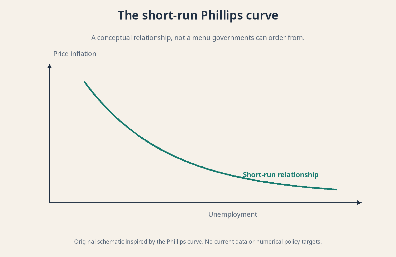
Original schematic inspired by the Phillips curve. No current data or numerical policy targets.
Why policymakers loved the apparent menu 🎛️
The tempting policy interpretation was a menu: support demand to reduce unemployment while accepting more inflation, or restrain spending to reduce inflation while accepting weaker employment. Demand here means spending by households, firms, government and external buyers. If the relationship were reliably stable, policymakers might appear able to select a combination.
The mistake is turning an observed association into a perfectly controllable machine. People adapt, contracts reset and the productive structure changes. Not every price movement begins with demand either. A menu that rearranges itself while you order is not much of a menu. Supply and expectations can change the choices available.
Nor does the curve mean high inflation should be pursued as a shortcut to prosperity. Spending persistently beyond productive capacity does not immediately train workers or build infrastructure. Prices can rise without preserving the initial employment gain. A temporary demand effect is not the same as sustainable productive improvement.
Friedman and Phelps: People don’t forget about inflation 🧠
In the 1960s, Milton Friedman and Edmund Phelps separately emphasized expectations. Workers and businesses don’t negotiate forever as if prices will stay unchanged. They try to anticipate inflation when setting wages and contracts. Expected inflation therefore belongs in the explanation, rather than being an optional detail added after drawing the curve.
Unexpected inflation can temporarily affect output and employment because some wages and contracts adjust slowly. Repeated surprises are harder to repeat: people incorporate the pattern into their expectations. In this framework, sustaining the same unemployment benefit would require further unexpected inflation, not simply a permanently higher but stable inflation rate.
In the diagram, higher expected inflation shifts the short-run curve upward: a given unemployment rate can coincide with more inflation. That differs from moving along an unchanged curve. Movement describes a change with the assumed background held fixed; a shift changes that background. Confusing them hides the central point of the expectations argument.
Short run vs. long run: Why a vertical line appears 📏
In the standard expectations-augmented model, no permanent long-run trade-off allows lower unemployment merely by selecting higher inflation. The long-run curve is drawn vertically at an equilibrium unemployment rate. This is a model result under assumptions, not a claim that every real-world adjustment is immediate or painless.
The natural rate represents unemployment consistent with the model’s labor-market structure and frictions. Natural does not mean desirable, biologically determined or impossible to change. Institutions, skills, mobility, information and matching processes influence it. Policies improving those features can affect employment differently from simply pushing aggregate demand harder.
NAIRU, the non-accelerating inflation rate of unemployment, is a related concept: the unemployment rate consistent with inflation not accelerating under the relevant assumptions. It is not identical to the natural rate in every model. Both are estimated with uncertainty, can change and cannot be read directly from a monthly statistical release.
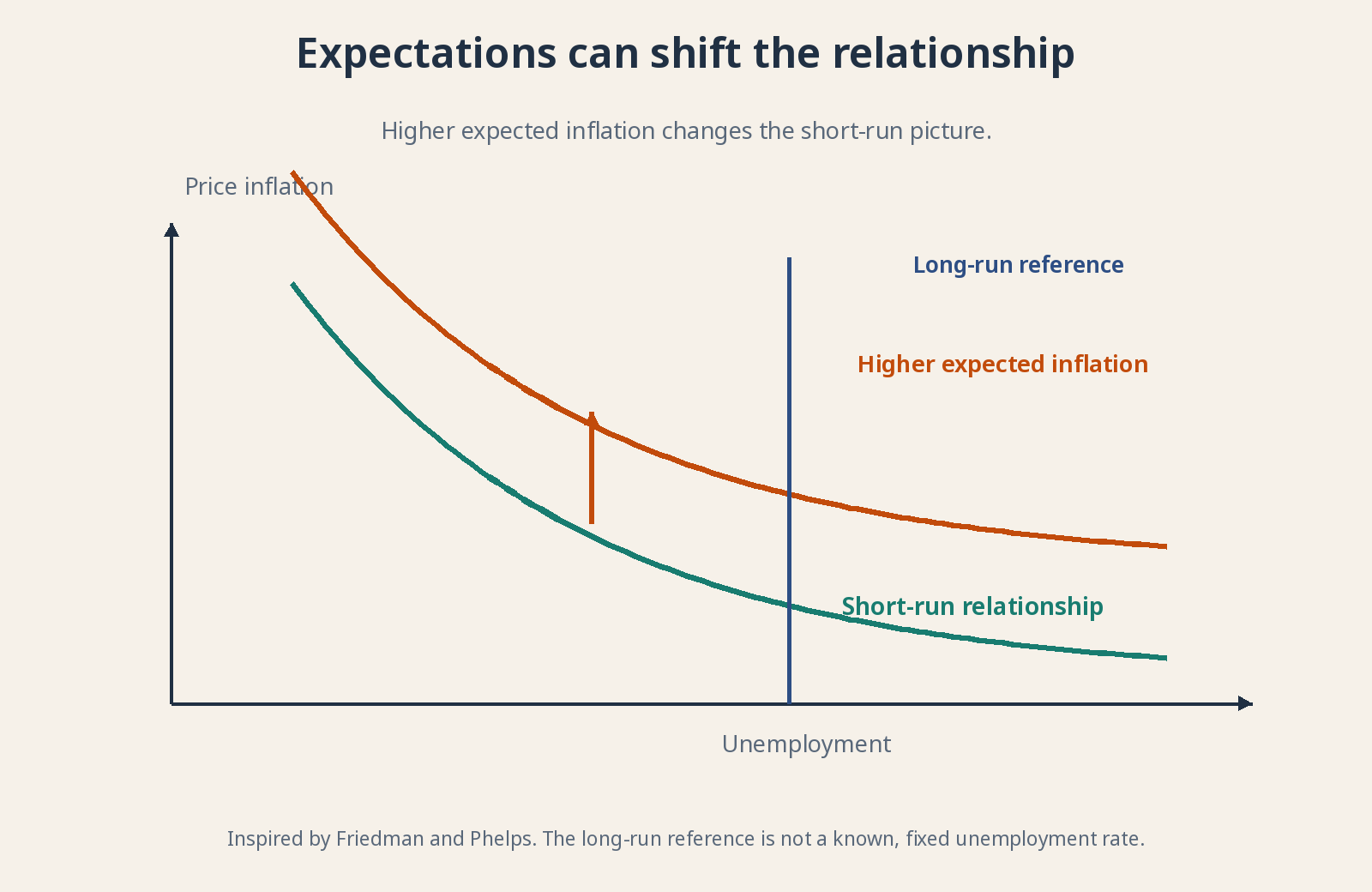
Conceptual diagram inspired by Friedman and Phelps. Inspired by Friedman and Phelps. The long-run reference is not a known, fixed unemployment rate.
Stagflation: When both rise together 🛢️
The stagflation episodes of the 1970s exposed the fragility of a fixed trade-off. High inflation coexisted with weak activity and labor-market difficulties. Oil shocks raised production costs, alongside other influences including expectations and policy. The economy did not politely remain on one tidy downward-sloping line.
When production becomes more expensive, firms may increase prices while cutting output and employment. The short-run curve shifts adversely: more inflation for a given unemployment rate, or worse employment at a given inflation rate. Both headline problems can worsen together without contradicting an account that allows supply conditions to change.
This connects to lesson 3.4. A central bank can restrain a shock’s propagation into spending and expectations, but higher rates do not manufacture oil. Ignoring inflation because it began with supply can still allow persistence to develop. Recognizing the source explains the dilemma; it does not make the policy response costless.
Productivity and margins: Wages aren’t the whole story ⚙️
Labor productivity measures output per unit of labor, such as per hour. If each hour produces more, higher wages can coexist with little change in labor cost per unit. Unit labor cost relates labor compensation to output. That is why a nominal wage rise alone cannot establish how much inflation pressure it creates.
Margins, competition and imported prices also matter. A firm facing weak sales may absorb higher costs; one with strong demand may pass more through. National averages conceal very different sectors and bargaining conditions. You cannot read the entire inflation process from one wage figure any more than you can assess a company from one invoice.
The ongoing debate: Useful, but neither position nor slope is fixed 🔍
Economists debate the curve’s slope, the role of expectations and imports, and whether responses intensify near capacity limits. A flatter curve means unemployment changes are associated with smaller inflation changes, other things equal. That does not automatically mean the mechanism has vanished; it can mean its observed strength depends on the period and conditions.
Nonlinearity means the relationship does not respond with the same intensity everywhere. Hiring one more worker may be easy with substantial spare capacity and difficult when many firms are recruiting simultaneously. Pressure can therefore intensify near bottlenecks. A straight line is convenient for a lesson, not a requirement imposed on the economy.
The empirical challenge is that expectations, supply and policy change together. A weak association in one chart does not prove the mechanism dead; a strong relationship in one period does not guarantee it will persist. Use the model to ask better questions, then compare it with evidence. Don’t ask a simple diagram to do the whole research department’s job.
Why does this matter to you as an investor? 📈
Because “lower unemployment” doesn’t translate into “good for every asset.” It may signal strong demand, but also cost pressure or tighter-than-expected monetary policy. Higher unemployment can ease certain pressures without offsetting damage to sales. The effect depends on context and what market prices already reflect.
Consider employment, participation, wages, productivity, margins and the composition of inflation together. Ask how they reach a company’s customers and costs—not which trade a curve commands. Over a long horizon, recognizing uncertainty is an advantage. It keeps a useful drawing from becoming an expensive certainty.
For further reading: Bank of England: Phillips and inflation expectations · Bank of England: changes in the Phillips curve.